I first came across the à trous algorithm when I was looking for a good edge avoiding filter for SSAO. Back then I was trying to code a demo. I had depth of field, some kind of hdr, spherical harmonics ambient lighting and screen space ambient transfer. I tried several techniques like the bilateral filter described in this paper (4.2 Bilateral Upsampling). I don’t remember why but I have issues with this filter so I went on a quest for a better filter. Long story short, thanks to Ke-Sen Huang’s page I read a paper called Edge-Avoiding A-Trous Wavelet Transform for fast Global Illumination Filtering (paper, slides).
I won’t make a lecture about wavelet transforms but this is how it roughly works.
We start with the source image I. At each iteration iwe will compute 2 images, \(d_i\) and \(c_i\). The first one will hold the filtered output and the second the details. This can be translated as:
- \(c_0 = I\)
- \(c_{i+1}(p) = \sum_{k \in H} h_i(k) c_i(p+2^ik)\)
- \(d_i = c_i – c_{i+1}\)
With \(h_i\) being the filter. And \(H\) the size of our filter. When the desired iteration \(n\) is reached, the set of detail images and the last filtered image form our wavelet transform.
- \(w(I) = \{d_0, d1, \cdots, d_{n-1}, c_n\}\)
As you can see, the space between each sample doubles at each iteration. Hence the name “à-trous” (with holes). Moreover the dimensions of the filtered images do not change. As opposed to Haar wavelet transform where \(c_{i+1}\) is half the size of \(c_i\).
The next step is called the synthesis. We simply add the elements of the \(w(I)\) to produce the final image.
- \(I’ = c_n + \sum_{0 \leq i < n}d_i\)
The wavelet filter can be seen as a pyramidal algorithm. The wavelet transform is the “pull” phase. And the synthesis the “push” phase (see this paper for an overview of “push pull” algorithm). As the scaling function is a \(B_3\) spline, the filter \(h\) is :
- \(\left(\frac{1}{16},\frac{1}{4},\frac{3}{8},\frac{1}{4},\frac{1}{16}\right)\) in \(\mathbb{R}\)
- \(
\begin{pmatrix}
\frac{1}{256} & \frac{1}{64} & \frac{3}{128} & \frac{1}{64} & \frac{1}{256} \\
\frac{1}{64} & \frac{1}{16} & \frac{3}{32} & \frac{1}{16} & \frac{1}{64} \\
\frac{3}{128} & \frac{3}{32} & \frac{9}{64} & \frac{3}{32} & \frac{3}{128} \\
\frac{1}{64} & \frac{1}{16} & \frac{3}{32} & \frac{1}{16} & \frac{1}{64} \\
\frac{1}{256} & \frac{1}{64} & \frac{3}{128} & \frac{1}{64} & \frac{1}{256}
\end{pmatrix}
\) in \(\mathbb{R}^2\)
If we apply this to image filtering, we will have:
- \(c_0 = I\)
- \(\forall i \in [0,n[\) and \(\forall p \in [0,S_x] \times [0,S_y[\)
- \(c_{i+1}(p) = \sum_{0 \leq y < 5} \sum_{0 \leq x < 5} h_i(x,y) c_i\left(p+ 2^i(x,y)\right)\)
- \(d_i(p) = c_i – c_{i+1}(p)\)
- \(I’=c_n + \sum_{0 \leq i < n}d_i\)
Edge awareness is acheived by adding a Gaussian distribution based weighing function of the colorimetric difference between the sample and source pixel (just like any standard bilateral filter).
- \(\omega_{\sigma}(u,v) = e^{\frac{\left\|c_i(u) – c_i(v)\right\|^2}{\sigma}}\)
2will be:
- \(c_{i+1}(p) = \frac{1}{W} \sum \sum \omega_{\sigma}\left(c_i(p),c_i\left(p+2^i(x,y)\right)\right)h_i(x,y) c_i(p+2^i(x,y))\)
- with \(W = \sum\sum \omega_{\sigma}\left(c_i(p),c_i\left(p+2^i(x,y)\right)\right)h_i(x,y)\)
Denoising can be acheived by thresholding the detail images.
- \(d’_i = max\left(0, |d_i|-\tau\right) \cdot sign(d_i)\)
More details can be found in “Edge-Optimized À-TrousWavelets for Local Contrast
Enhancement with Robust Denoising” by Johannes Hanika, Holger Dammertz and Hendrik Lensch (paper, slides).
Implementing it in OpenGL/glsl is pretty straightforward. The detail textures will be stored in a texture array. And as we only need the last filtered image for the synthesis, we will ping-pong between 2 textures.
Here is how the texture array is created:
glBindTexture(GL_TEXTURE_2D_ARRAY, texId);
	glTexImage3D(GL_TEXTURE_2D_ARRAY, 0, GL_RGB32F, imageWidth, imageHeight, LEVEL_MAX, 0, GL_RGB, GL_UNSIGNED_BYTE, 0);
	for(i=0; i<LEVEL_MAX; i++)
        {
		glTexSubImage3D(GL_TEXTURE_2D_ARRAY, 0, 0, 0, i, imageWidth, imageHeight, 1, GL_RGB, GL_UNSIGNED_BYTE, imageData);
	}
	// Set texture wrap and filtering here.
glBindTexture(GL_TEXTURE_2D_ARRAY, 0);
You attach a layer just like a standard 3D texture.
glBindFramebuffer(GL_FRAMEBUFFER, framebuffer);
glFramebufferTextureLayer(GL_FRAMEBUFFER, GL_COLOR_ATTACHMENT0, texId, 0, layerIndex);
You access it in a shader using a sampler2DArray. Here is an example based on the synthesis shader:
#extension GL_EXT_texture_array : enable
uniform sampler2D filtered;
uniform sampler2DArray details;

out vec4 outData;

void main()
{
    int levelMax = int(textureSize(uDetails, 0).z);
    vec4 data = texelFetch(filtered, ivec2(gl_FragCoord.xy), 0);;

    for(int i=0; i<levelMax; i++)
    {
		data += texelFetch(details, ivec3(gl_FragCoord.xy, i), 0);
    }

    outData = data;
}
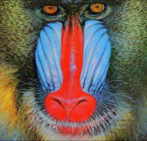
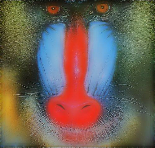
I uploaded the source code of a little demo here. It will filter the infamous mandrill image using a edge preserving à-trous wavelet transform. I intentionally used “extreme” parameters to show the effects of the edge avoiding filter. It comes with a Microsoft Visual Studion 2010 project. Note that you will need GLFW and GLEW. You will also have to edit the ContribDir item in platform\windows\wavelet.vcxproj.props.
On the left you have the original image. And on the right the filtered image with \(\sigma=1.125\) and \(\tau=0.05125\).


Stuffs
References
- Gilbert Strang, Lecture 27: Multiresolution, wavelet transform and scaling function
- Albert Bijaoui, Jean-Luc Starck, Fionn Murtagh, Restauration des images multi-échelles par l’algorithme à trous (french)
- Holger Dammertz, Daniel Sewtz, Johannes Hanika, Hendrik P.A. Lensch, Edge-Avoiding À-Trous Wavelet Transform for fast Global
Illumination Filtering, (slides) - Johannes Hanika, Holger Dammertz, Hendrik Lensch, Edge-Optimized À-Trous Wavelets for Local Contrast Enhancement with Robust Denoising, (slides)
- Peter-Pike Sloan, Naga K. Govindaraju, Derek Nowrouzezahrai, John Snyder, Image-Based Proxy Accumulation for Real-Time Soft Global Illumination
- Martin Kraus, The Pull-Push Algorithm Revisited


