Tag: image processing

What is an image histogram?
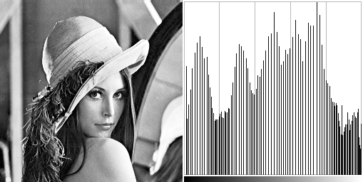
Well, it is fairly simple. Consider we have a grayscale image. Its histogram is an array that stores the number of occurence of each grey level. It gives us a representation of the tone distribution.

If an image is dark, there will be a peak near the lowest tone values. Or the other hand brighter image will have peaks near the maximum tone values.

The image histogram can also give us informations about its contrast. An image with a low contrast will have a peak around its median value and most of the histogram values will be concentrated around that peak. Alternatively a highly contrasted image will have peaks around its minimal and maximal tone value as long as sparse low values in between.

It seems logical that if we stretch the histogram over the whole tone range, we will increase the image constrast. This operation is called histogram equalization. Before going any further, let’s introduce some basic definitions. The first one is the probability density function:

\(P^{[l_s,l_f]}_l = \frac{h_l}{H^{[l_s,l_f]}}\)

With \(0 \le l_s < l_f \le l_{max}[/latex]. Usually [latex]l_{max} = 255[/latex].

[latex]H^{[m,n]}\) is introduced for brevity. It’s the sum of the histogram value over the range \([m,n]\).

\(H^{[m,n]} = \sum_{i=m}^{n}h_i\)

Next is the probability distribution function.

\(C^{[l_s,l_f]}_l = \frac{\sum_{i=l_s}^{l}h_i}{H^{[l_s,l_f]}}\)

Which can be rewritten as:

\(C^{[l_s,l_f]}_l = \sum_{i=l_s}^{l}P^{[l_s,l_f]}_i\)

The mean of the histogram values is also called the image brightness.

\(l_m = \frac{\sum_{i=l_s}^{l_f}i \times h_i}{H^{[l_s,l_f]}}\)

To put it simply,

\(l_m = \sum_{i=l_s}^{l_f}i P^{[l_s,l_f]}_i\)

The aim of histogram equalization is to produce a histogram where each tone has the same number of occurence (uniform distribution). This is equivalent to saying that any tone \(l\) has the same density.

\(P’^{[l_s,l_f]}_{l} = \frac{1}{l_f – ls}\)

Which gives us the ideal probability distribution function.

\(C’^{[l_s,l_f]}_{l} = \sum_{i=l_s}^{l}P’^{[l_s,l_f]}_i = \frac{l-ls}{lf – ls}\)

A way to acheive this is to find \(l’\) that minimizes the difference between \(C’^{[l_s,l_f]}_{l’}\) and \(C^{[l_s,l_f]}_{l}\). In other words, we want to find \(l’\) so that:

\(C^{[l_s,l_f]}_{l} = C’^{[l_s,l_f]}_{l’}\)

Which gives us:

\(l’ = l_s + \big\langle(l_f – l_s) C^{[l_s,l_f]}_l \big\rangle\)

Where \(\langle x \rangle\) is the nearest integer to \(x\).

This technique is sometimes referred as the classical histogram equalization or CHE. The drawback of this method is that it changes the image brightness.

The following source code is performing CHE with \(ls = 0\) and \(l_f = l_{max}\).
This code is using the CImg library.

    // We will load a dark grayscale version of the 
    // classical lena image.
    CImg<unsigned char> source;
    source.load("dark_lena.png");
	
    unsigned long int lut[256];
    unsigned long int histogram[256];

    // Build image histogram.
    memset(histogram, 0, sizeof(unsigned long int)*256);
    cimg_forXY(source, x, y)
    {
        histogram[source(x,y,0,0)]++;
    }

    // Compute probality distribution function.
    unsigned long int sum = 0;
    for(int i=0; i<256; i++)
    {
        sum += histogram[i];
        lut[i] = floor(255.0 * sum / (source.width() * source.height()) + 0.5);
    }
    
    // Perform CHE
    cimg_forXY(source, x, y)
    {
        source(x,y,0,0) = lut[(int)source(x, y, 0, 0)];
    }
  

References:

• David Menotti Gomes. Contrast Enhancement in Digital Imaging using Histogram Equalization. PhD Thesis, June 2008

I recently played with median cut quantization. Like octree quantization, color space is viewed as a 3D space. But it uses a top-bottom approach. We start with a box containing all the image colors and then we split it into 2 smaller boxes along its longest side until the number of boxes is equal to the number of desired colors. The child boxes are then shrunk to enclose their color subset. Each color in the palette is then the mean of the colors contained in each box.
I used stl priority queue to store the boxes and get the box with the longest side. As each new box contains half of its parent color. The first subset contains all the colors where the component along the split axis is inferior to the median. And on the other hand, the second subset color component along the split axis are greater than the median. For this i use the nth_element function.
I should have used them for the octree quantization…
Talking about octree, i put all the image colors into one in order to easily map them to the palette.

The result is quite good with the sorcerian images.

Here’s the RGB color wheel. The error is very important for low color count 🙁

truecolor	256
128	64
32	16

I tried to solve this problem by spliting the box along the axis with the highest variance. But the result is not that great.

Anyway! Grab the sources here.

I’m currently reading a paper about using Kohonen neural networks for color quantization. I think i’ll implement median cut before starting implementing it. This way i’ll can’t compare it with something other than my current octree implementation.

Talking about the octrees! In the last post, the artifacts where caused by the fact that i didn’t merge the node with the least pixel count. In fact, i was merging the last created node. This was clearly visible for the 32 colors version of the RGB color wheel.

I added the pixels to the octree this way:

for(j=0; j<h; ++j)
{
    for(i=0; i<w; ++i)
    {
        octree.add(pixel[i][j]);
    }
}

The gradient is more detailed for pixel near the origins (the first pixel inserted). In the following image, the pixels are inserted in backward order (from (w,h) to (0,0)). We see that the gradient is inverted (just as we thought).

Here’s the result with pixels inserted in random order. The gradient artifact seems to have disappear. But the result still isn’t correct as we don’t respect the standard merge criteria.

The only thing to do is to sort the mergeable nodes according to their pixel count. As a list is stored for each octree level, a merge sort sounds the best solution. I’m using this implementation as i’m not using the STL. The gradient disappears for the RGB colorwheel, but the sorcerian image colors are still washed out…

And here’s the source code.

The last 3 days (nights…), I played with octree color quantization. It’s another use of hierarchical data structure for computer graphics.

We first contruct the octree (a tree where each node as at most 8 children) by inserting each image color in it. Let’s assume that the color is encoded in 24 bits (8bits per component). The octree has then 8 levels. So, we first take the
most significant bit of each component and merge them to obtain the child index.

shift = 7 - level;
child = (((red >> shift) <<  2) & 0x04) | (((green >> shift) <<  1) & 0x02) | ((blue >> shift) & 1);

A leaf is contructed when we reach the first bit. The current color is added to the leaf color and a reference counter is incremented (it’s basically counting the color occurence in the image).

Then the leaves are successively merged until we reach the desire color count.

node = node to be merged
for(i=0; i<8; ++i) {
    if(node->child[i]) {
        node->rgb += node->child[i]->rgb;
        node->reference += node->child[i]->reference;
        delete(node->child[i]);
    }
}

The original paper stated that the nodes with the least number of pixels (the lowest reference count) must be merged first. Actually, I’m keeping an array containing the node list (newly created node is inserted at the head) for each level. Then i backward traverse this tree from the bitCount-1 (here 7th, as the 8th entry contains the leaves list) and merge each node in the list until i reach the desired color count. This is clearly unoptimal.
Thereafter, the palette entries are built by taking each leaf color and dividing it by its reference count. The indexed image is then built by taking each color and traverse the octree. The index of the pixel color is the one of the leaf color we reach.

Here’re some results! The following table show the quantization of a 24bpp rgb color wheel.

256	128
32	16

The artifact generated by the current merge criteria (merge the last created node for the current level) is clearly visible. I should make some kind of priority queue and then merge the node with the lowest priority (this reminds me the ROAM algorithm for terrain rendering).The following image is a sample of a Sorcerian wallpaper reduced to 16 colors. Here the lazy merge criteria flattens the colors.

Here’s the same image reduced to 16 colors using GIMP (without dithering). It seems that GIMP uses the median cut method.

I will fix the merge criteria right now. I think i’ll implement color quantization using Kohonen neural networks first.
Meanwhile, here’s the source code.