


The last 3 days (nights…), I played with octree color quantization. It’s another use of hierarchical data structure for computer graphics.
We first contruct the octree (a tree where each node as at most 8 children) by inserting each image color in it. Let’s assume that the color is encoded in 24 bits (8bits per component). The octree has then 8 levels. So, we first take the
most significant bit of each component and merge them to obtain the child index.
shift = 7 - level;
child = (((red >> shift) <<  2) & 0x04) | (((green >> shift) <<  1) & 0x02) | ((blue >> shift) & 1);
A leaf is contructed when we reach the first bit. The current color is added to the leaf color and a reference counter is incremented (it’s basically counting the color occurence in the image).
Then the leaves are successively merged until we reach the desire color count.
node = node to be merged
for(i=0; i<8; ++i) {
    if(node->child[i]) {
        node->rgb += node->child[i]->rgb;
        node->reference += node->child[i]->reference;
        delete(node->child[i]);
    }
}
The original paper stated that the nodes with the least number of pixels (the lowest reference count) must be merged first. Actually, I’m keeping an array containing the node list (newly created node is inserted at the head) for each level. Then i backward traverse this tree from the bitCount-1 (here 7th, as the 8th entry contains the leaves list) and merge each node in the list until i reach the desired color count. This is clearly unoptimal.
Thereafter, the palette entries are built by taking each leaf color and dividing it by its reference count. The indexed image is then built by taking each color and traverse the octree. The index of the pixel color is the one of the leaf color we reach.
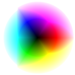
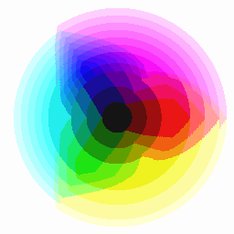
Here’re some results! The following table show the quantization of a 24bpp rgb color wheel.
 |
|
 |
 |
| 256 | 128 |
 |
 |
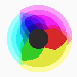
| 32 | 16 |
Here’s the same image reduced to 16 colors using GIMP (without dithering). It seems that GIMP uses the median cut method.
I will fix the merge criteria right now. I think i’ll implement color quantization using Kohonen neural networks first.
Meanwhile, here’s the source code.

")