Color blasting (part 3)

I recently played with median cut quantization. Like octree quantization, color space is viewed as a 3D space. But it uses a top-bottom approach. We start with a box containing all the image colors and then we split it into 2 smaller boxes along its longest side until the number of boxes is equal to the number of desired colors. The child boxes are then shrunk to enclose their color subset. Each color in the palette is then the mean of the colors contained in each box.
I used stl priority queue to store the boxes and get the box with the longest side. As each new box contains half of its parent color. The first subset contains all the colors where the component along the split axis is inferior to the median. And on the other hand, the second subset color component along the split axis are greater than the median. For this i use the nth_element function.
I should have used them for the octree quantization…
Talking about octree, i put all the image colors into one in order to easily map them to the palette.

The result is quite good with the sorcerian images.

Sorcerer images (median Cut 16 colors)

Here’s the RGB color wheel. The error is very important for low color count 🙁

RGB Color Wheel RGB Color Wheel (median cut 256 colors)
truecolor 256
RGB Color Wheel (median cut 128 colors) RGB Color Wheel (median cut 64 colors)
128 64
RGB Color Wheel (median cut 32 colors) RGB Color Wheel (median cut 16 colors)
32 16

I tried to solve this problem by spliting the box along the axis with the highest variance. But the result is not that great.

Sorcerer images (median Cut 16 colors variance)

Anyway! Grab the sources here.

Color blasting (part 2)

I’m currently reading a paper about using Kohonen neural networks for color quantization. I think i’ll implement median cut before starting implementing it. This way i’ll can’t compare it with something other than my current octree implementation.

Talking about the octrees! In the last post, the artifacts where caused by the fact that i didn’t merge the node with the least pixel count. In fact, i was merging the last created node. This was clearly visible for the 32 colors version of the RGB color wheel.

RGB Color Wheel (32 colors)

I added the pixels to the octree this way:

for(j=0; j<h; ++j)
{
    for(i=0; i<w; ++i)
    {
        octree.add(pixel[i][j]);
    }
}

The gradient is more detailed for pixel near the origins (the first pixel inserted). In the following image, the pixels are inserted in backward order (from (w,h) to (0,0)). We see that the gradient is inverted (just as we thought).
Colorwheel (32 colors) north west

Here’s the result with pixels inserted in random order. The gradient artifact seems to have disappear. But the result still isn’t correct as we don’t respect the standard merge criteria.

Colorwheel (32 colors) random

The only thing to do is to sort the mergeable nodes according to their pixel count. As a list is stored for each octree level, a merge sort sounds the best solution. I’m using this implementation as i’m not using the STL. The gradient disappears for the RGB colorwheel, but the sorcerian image colors are still washed out…

Sorcerian image 16colors with octree quantization

And here’s the source code.

Color blasting

The last 3 days (nights…), I played with octree color quantization. It’s another use of hierarchical data structure for computer graphics.

We first contruct the octree (a tree where each node as at most 8 children) by inserting each image color in it. Let’s assume that the color is encoded in 24 bits (8bits per component). The octree has then 8 levels. So, we first take the
most significant bit of each component and merge them to obtain the child index.

shift = 7 - level;
child = (((red >> shift) <<  2) & 0x04) | (((green >> shift) <<  1) & 0x02) | ((blue >> shift) & 1);

A leaf is contructed when we reach the first bit. The current color is added to the leaf color and a reference counter is incremented (it’s basically counting the color occurence in the image).

Then the leaves are successively merged until we reach the desire color count.

node = node to be merged
for(i=0; i<8; ++i) {
    if(node->child[i]) {
        node->rgb += node->child[i]->rgb;
        node->reference += node->child[i]->reference;
        delete(node->child[i]);
    }
}

The original paper stated that the nodes with the least number of pixels (the lowest reference count) must be merged first. Actually, I’m keeping an array containing the node list (newly created node is inserted at the head) for each level. Then i backward traverse this tree from the bitCount-1 (here 7th, as the 8th entry contains the leaves list) and merge each node in the list until i reach the desired color count. This is clearly unoptimal.
Thereafter, the palette entries are built by taking each leaf color and dividing it by its reference count. The indexed image is then built by taking each color and traverse the octree. The index of the pixel color is the one of the leaf color we reach.

Here’re some results! The following table show the quantization of a 24bpp rgb color wheel.

RGB Color Wheel
RGB Color Wheel (256 colors) RGB Color Wheel (128 colors)
256 128
RGB Color Wheel (32 colors) RGB Color Wheel (16 colors)
32 16

The artifact generated by the current merge criteria (merge the last created node for the current level) is clearly visible. I should make some kind of priority queue and then merge the node with the lowest priority (this reminds me the ROAM algorithm for terrain rendering).The following image is a sample of a Sorcerian wallpaper reduced to 16 colors. Here the lazy merge criteria flattens the colors.
Piece of sorcerian wallpaper in 16 colors

Here’s the same image reduced to 16 colors using GIMP (without dithering). It seems that GIMP uses the median cut method.
Sorcerian wallpaper 16 colors (gimp)
I will fix the merge criteria right now. I think i’ll implement color quantization using Kohonen neural networks first.
Meanwhile, here’s the source code.

Plückermeister

I replaced the Möller ray/triangle intersection test by the one using Plücker coordinates. It’s faster and more robust. The results is looking better (smoother normals). But, the holes didn’t disapear. After some investigations, i discovered that the problem came from point normals (I’m using them as point color). I read the objects from ply2 files which only store points and polygon indexes. Here’s how i’m computing point normals:

v is the mesh vertex list
n is the mest point normal list
foreach triangle t
    t.n = normalize(cross(v[t.p1]-v[t.po],v[t.p2]-v[t.po]))
    n[t.p0] += t.n
    n[t.p1] += t.n
    n[t.p2] += t.n
normalize each n

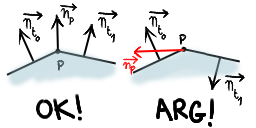
There’s a huge problem here. We are assuming that each polygon (triangle in this case) are ordered so that its normal is pointing away from the object. Unfortunately, this isn’t guaranteed by ply2 format. The following figure illustrates this.

Mesh normal problem

Imagine if t0 and t1 are coplanar. If we are in the worst case, the normals of t0 and t1 are pointing in the opposite directions. As the normal at p is the sum of those two normals, it’ll be equal to the null vector. That explains the black holes. But that’s not all… The normal at the intersection point between the ray and the triangle is interpolated from the point normals of the triangle using barycentric coordinates. One of these 3 normals may be wrong or/and, like the figure, they may be pointing in opposite directions… Arg!

There’s no exact way to determine if a polygon normal is pointing away from the surface. So, unless the file format provides polygon (or in the best case) points normals, i’ll not interpolate point normals.

Enter the dragon

I backported the BVH i wrote for CRBN to the little and ugly raytracer test. Even if it’s not the most efficient space partioning method for raytracing, the improvment is quite impressive.

Here’re some results with the Maneki Neko model rendered on a Athlon XP 1.4GHz with 1GB of RAM. The model contains 62385 points and 124677 triangles. The code was compiled only with the -O flag and the target image was 256×256.

BVH:
  • real 0m8.325s
  • user 0m6.461s
  • sys 0m1.505s
  • 174 MB
Without:
  • real 25m57.370s
  • user 24m25.249s
  • sys 0m5.714s
  • 52MB

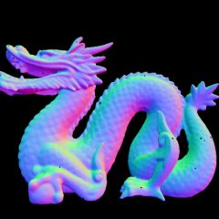
Nice heh? So i decided to render something a little bit bigger. I chose the dragon hi-res model. It contains 437645 vertices and 871414 triangles. I haven’t tried rendering it without BVH. The 512×512 image took 2minutes to render. Unfortunately, i still have some floating point issues. You can notice holes here and there… I’ll made some tests using Plüecker coordinates as it’s supposed to be more robust.
Dragon (small)

8bit archeology

Some years ago, i wrote a very simple and stupid pcengine disassembler in order to check if the rom i produced with wla-dx were correct. Well, time fly and two weeks ago i dig it from the grave. The user can now specify which part of the pcengine rom will be disassembled (code section) and which one are pure data. For this i’m using a csv file. The whole thing is discribed in the README file i quickly wrote tonight 🙂

I started coding it under Linux. As i was in a hurry and lazy, i decided to mmap the rom file. But unfortunately, mmap is not supported/implemented by mingw32. So i had to use my mighty google skills (well koders ones in this case). And the same thing happened with the CSV file parser. I’m using strndup and… i had to recode it :/

Enought ranting! I put everything THERE . The directory contains the complete source code, makefiles for both windows and linux, windows binary and the dev C++ project. As an example, i disassembled Momotaro Desentsu Turbo . I started to document the reset interrupt.

Buddah ray

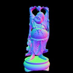
I decided to render a larger model. So i took the happy buddah model from stanford repository. It contains 543652 points and 1087716 triangles. Rendering a 256×256 image took approximatively 2 hours. I really need surface partitioning.

The white dots on the picture represent the ray where a floating point error occured. As the mesh has really small triangles and low coordinates points, i had to replace the zero divider test using boundaries by the standard not equal to zero test. I really hate this floating point issues…

Budda (small)

Raytracing beeps

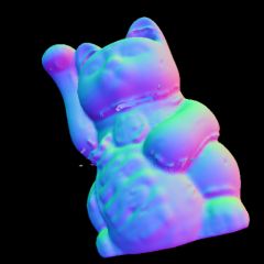
I quickly wrote some basic polygonal mesh raytracer in order to test some space partitioning algorithm like KD-trees or BIH. I’m actually using the maneki neko from this repository. It’s not really big compared to stanford bunny or happy buddha. As i don’t need any lighting, i decided to use point normal as color. Here’s the result :

Maneki Neko (small)

It took 25 minutes to render this image on my amd64 3500+. The model contains 62385 points and 124677 triangles. Not that much… But it’s brute force raytracing for the moment.
I also discovered that XYZ-RGB is offering free texture materials. Maybe i should use them for the displacement map.

On the 8bit side, the pcengine tracker is going well. The instrument routines may be finished next week. Next step is note/pattern handling.

Triangle Slicing part 2

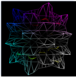
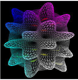
I finally manage to make displacement mapping work. Here are the results for level 8 and 32 subdivisions. Vertex texture fetch seems to be slow on my card (6600 gt).

I need to check if my code is really optimal (well i’m pretty sure it isn’t 🙂 ). But for now, i’m leaving for vacation for 2 weeks!

8 32
Vertex texture fetch 8 Vertex texture fetch 32

Triangle Slicing

Thanks to a java/firefox crash combo, i lost the article i was writing. So here’s a shortened version without all the explanation (i’ll write them later).

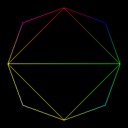
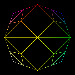
Last week, I came across a paper called “Generic Mesh Refinement on GPU” and decided to implement it. I finished the refinement pattern generation and the use of a vertex shader to display the refined mesh today.
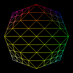
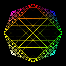
Here are the results:

1 2
Level 1 refinement Level 2 refinement
4 8
Level 4 refinement Level 8 refinement

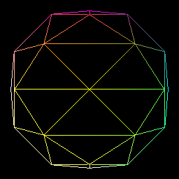
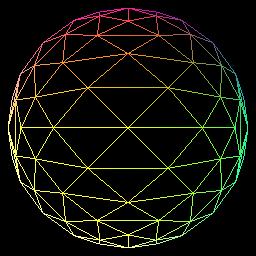
As my main goal is to use this technique for displacement mapping, i modify each point in order to map a sphere:

1 2
Level 1 refinement Level 2 refinement (sphere)
4 8
Level 4 refinement (sphere) Level 8 refinement (sphere)