Zero right ahead!

Yes! Zero wouldn’t be considered as the default/standard return error value. I learnt the hard way today.

I had some kind of weird NULL pointer bug. After some investigations, i found that the deserialization function was failing at some point leaving the whole structure uninitialized. First i blamed myself for not calling the standard structure initialization function when the deserialization function failed. Then i looked at the data file.
Everything seemed to be ok. So i went on a step by step execution with the debugger. 5 minutes later i found the culprit. It was zlib in the kitchen with ten tone hammer. It was strange.

Let’s say that i compressed a buffer of N bytes into M bytes. When i read back the N bytes from the compressed buffer, i get the whole data before the end of the compressed buffer. Leaving me with 5 extra bytes.
On the next run i try to read P bytes. But i still have those 5 bytes to decompress. So i feed them to inflate (the zlib decompression routine). It returns a nice Z_STREAM_END. At this point, nothing wrong as i finished to process the previous compressed buffer. But (and that’s a big but     …     sorry    ) no bytes were output.
In fact it’s an excellent news as we already get the N bytes back. So this bytes are … what… padding bytes ?
Anyway, the fact that i got 0 bytes back without any zlib or system error was a relief. But the “dezip” function is returning 0 on error or the size of the decompressed data when everything works…
So… I was considering that the “dezip” function failed even if everything was alright.

The whole issue was fixed in 5 minutes by changing the default error value from 0 to -1….

I spent the whole day tracking this bug…

The Attack of the Patatoids!

Last day i was reading the wikipedia article about the Pioneer program. I don’t know how, but after following some links i ended on the Hayabusa mission article.
The Hayabusa space probe was launch in 2003 to study the Itokawa asteroid. The most ambitious part of the mission was about landing on the astoreid to collect samples. From what i understood, the samples would not have been collected by drilling the asteroid but from the debris made by the collision between the asteroid and a projectile launched from the space probe. Unfortunately, the attempts to land on the asteroid failed. Nevertheless, it seems that the Hayabusa managed to collect some samples.
The Hayabusa may be bak to earth around 2010.

Using the data collected, Robert Gaskell from the Planetary Science Institute generated 3D models of the Itokawa asteroid. The model is available in 3 formats (plate-vertex table, STL ASCII and triangle) and in 4 resolutions (from 49,152 to 3,145,728 triangles).
The plate-vertex table format is similar to ply2 format. So, i took the 3M triangles version. Translated it into ply2 and launched my crappy raytracer on it.
I was surprised by the rendering speed. A 256×256 image was rendered in less than 1 minute. Nevertheless, i had a nasty bug 🙁

Buggy rendering of Itokawa asteroid

As you may have noticed there’s a bug on the left part. Here’s a close up.

buggy correct
Buggy rendering of Itokawa asteroid (close up) Correct rendering of Itokawa asteroid (correct)

The “correct” image was obtained after 3 hours of computation by disabling BVH. So the problem came from the BVH code. After almost rewriting the BVH building and intersection code, i still had the same bug. Some heavy code review later, i realized that the wrong ray intersection was returned. In fact it was the informations of the last intersection instead of the one from the closest intersection point. It’s a very stupid bug. Well at least i cleaned up the BVH code.
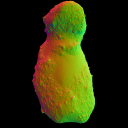
So for your pleasure here is a nice 512×512 image of the Itokawa asteroid.

512×512 image of Itokawa asteroid

And some stats:

  • BVH building time : 0h 0min 38.943722 sec
  • Rendering time : 0h 0min 7.411200 sec

As i said before, the code is greatly unoptimized but it manages to render a 3M triangles model in less than one minute. I’ll try to speed up the BVH building code, use a clever cost function and monitor memory usage (while running the top command, i noticed that more than 70% of the RAM (1go) was used.)

Bonus : dark side of the patatoid!

Dark side of the Itokawa asteroid

Having fun with OpenGL

This weekend i played a little bit with OpenGL. First, i helped my brother with some issues using the GL_ARB_texture_rectangle extensions. I never used it before. It’s very easy to use. You just have to use GL_TEXTURE_RECTANGLE_ARB instead of GL_ GL_TEXTURE_2D when you call openGL texture functions (or when you want to enable / disable texturing). The tricky part is that you have to specify that the pixel elements are stored one after the one. Also, textures coordinates values (u,v) are between [0,twidth]x[0,theight] instead of [0,1]x[0,1].

// Enable non rectangular textures
glEnable( GL_TEXTURE_RECTANGLE_ARB );
// Generate texture id
glGenTextures( 1, &id);
// Pixel component are stored linearly
glPixelStorei( GL_UNPACK_ALIGNMENT, 1 );
// And now store the texture data
glBindTexture( GL_TEXTURE_RECTANGLE_ARB, id);
glTexParameteri( GL_TEXTURE_RECTANGLE_ARB, GL_TEXTURE_MIN_FILTER, GL_LINEAR );
glTexParameteri( GL_TEXTURE_RECTANGLE_ARB, GL_TEXTURE_MAG_FILTER, GL_LINEAR );
glTexImage2D( GL_TEXTURE_RECTANGLE_ARB, 0, GL_RGB, textureWidth, textureHeight, 0, GL_RGB, GL_UNSIGNED_BYTE, data );

I must admit that i only used it to display a rectangular texture on screen. I found several examples on the web where it was used to avoid to scale the framebuffer when you save it to a texture.

As one of the GGI gsoc student is working on libggigl, i decided to code a little GLX example so that i don’t look stupid if he had questions about it 🙂
Here it is!
There’re no functions, no structures. Everything is the main. That’s what I call pigforce coding.
If I have time, I’ll try to play with offscreen rendering with GLX.

PCEngine tracker status : I’m writing code for hsync and vsync interrupts. It’s mostly a cleanup/study of mkit code. I hope to finish them this week and then start with tile/map management.

Captain’s clog

Aouch… 3 months since last post.
A lot of things happened. First of all i changed job (who said lame excuse?). Then GGI was selected for google summer of code. Guess who is the GGI admin on gsoc.. me :). 2 projects from the idea list were “slotted”. This means that google will fund them. The project i was about to mentor wasn’t selected. Anyway, i hope everything will be alright because some of the selected projects are part of the 3.0 roadmap.
Still about GGI, my current task is to implement Xdbe helper for X target. The task is not easy as it seems. My first try was kinda simplistic and … buggy. Instead of increasing X target speed, it slowed it down. And worst of all, i totally misunderstood the goal of Xdbe helper. It’s not just about swapping the window drawable. In fact, it’s the last and final part of the job. For the moment in X target, all the drawing operation are performed on the window drawable. Multiple buffering is performed by using window clipping. Let’s say we want a visual of 320×240 pixels and 3 frames (in order to do triple buffering, or whatever). We create a parent window with a size of 320 by 240. Then we create a child window of 320 x 240*3. We display a given frame by moving the child window so that the required area becomes visible.
For example, if we want to view the second frame, we move the child window by (0,240).
Back to Xdbe. We don’t need to use window auto-clipping anymore. We can use a single window with a backbuffer attach to it. If we want multiple frames, we can create a pixmap the same way we created the child window or create a pixmap per frame. All the drawing operations will be perfomed on the pixmap. Then on flush, we copy the pixmap data to the backbuffer and swap the window. It’s not as easy as it sounds because i’ll have to reorganize (or completly rewrite) the X target.

On the crbn/ray tracing front. There’s not much coding going on but i’m reading a lot… Ok. Let me rephrase it… I have a lot of papers and books to read 🙂

The pcengine tracker development was resumed this week. I hope to release a test rom for the instrument editor before the end of the month.

And now something different. Yesterday (and today) i rewrote the gallery with javascript and css. The old one was in perl/cgi and had a small oneliner. I still have the code lying around. I’d better burn it for the sake of mankind 🙂 However the only dynamic part in the new one is the image display in javascript, and as i now have this wonderfull blog, i threw the onliner away.
I put a link (“Doodles, drawings, sketch dump…”) to it in the section “My other stuffs”.

Typo negative

I cleaned up the 5×7 font rendering routine. It now uses mkit macros and variables. Here’s a little example of how to use it:

; set string length
lda    #28
sta    <_al

; set string pointer (don't forget to map it before)
lda    #low(string)
sta    <_si
lda    #high(string)
sta    <_si+1

; set vram address where the font will be rendered
lda    #$00
sta    <_di
lda    #$10
sta    <_di+1

; Here we go!
jsr    print5x7

; You can set BAT using the zp var _block containing
; the number of 8x8 bloc written

The code contained in the archive doesn’t need mkit as all the needed macros and variable declarations are included. If you want to use the font rendering with mkit, you’ll only have to include print5x7.asm and font.inc. font.inc contains both the standard 8×8 font, the 5×7 font and datas needed by the font routine.

You can download the archive [HERE].

Shrinked the glyph

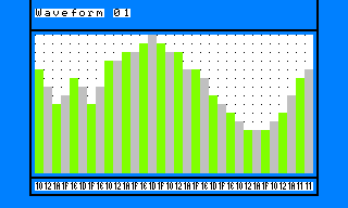
I made some mockups for the tracker interface using tile studio. It helped me realize that the standard 8×8 font might be too big. Here’re test images for the instrument and waveform editors.


Instrument editor interface

Waveform editor interface

As you can see, the 8×8 font used in the instrument editor menu is too big. The screen is 320×224 wide and i need to have an area of 256 pixels for the sequence editor. So one way to space is to use a smaller font. I decided to use 5×7 font. But there’s a problem. It’s easy to use 8×8 font as pcengine stores background graphics using 8×8 tiles. And these tiles are displayed using an array (a map). So if you want to print text, all you have to do is to store the font in VRAM and then set the map so that it points to the correct 8×8 tile. The code looks looks more or less like this (in fact it’s a little more complicated or pcengine) :

for(i=0; i<strlen(str); ++i)
{
    tile[x+i][y] = mapBaseAddress + 8 * ((x+i) + (y * W));
}

On the other hand, you can’t use the background tile map for 5×7 as it doesn’t fit the 8×8 boundary 🙁 So all we have to do is to render each text in vram. We’ll have to brutally concatenate bits.
In order to keep things a little bit optimized, i decided to unroll the concatenation loop for 8 iterations. Why? Erm… A little example will explain it better than i will.

byte 0: a0 b0 c0 d0 e0 a1 b1 c1
byte 1 d1 e1 a2 b2 c2 d2 e2 a3
byte 2: b3 c3 d3 e3 a4 b4 c4 d4
byte 3: e4 a5 b5 c5 d5 e5 a6 b6
byte 4: c6 d6 e6 a7 b7 c7 d7 e7

This table represents the output of the concatenations of 8 five bits values. We may repeat this for every 8 characters in the string and we’ll be done … 🙂 The following 2 images show the same string rendered with 8×8 and 5×7 fonts (clic them for a x2 zoom).


8x8 font example

5x7 font example

Here’s a marvelous rom demonstrating this breakthrough in computer science 🙂

Color blasting (part 3)

I recently played with median cut quantization. Like octree quantization, color space is viewed as a 3D space. But it uses a top-bottom approach. We start with a box containing all the image colors and then we split it into 2 smaller boxes along its longest side until the number of boxes is equal to the number of desired colors. The child boxes are then shrunk to enclose their color subset. Each color in the palette is then the mean of the colors contained in each box.
I used stl priority queue to store the boxes and get the box with the longest side. As each new box contains half of its parent color. The first subset contains all the colors where the component along the split axis is inferior to the median. And on the other hand, the second subset color component along the split axis are greater than the median. For this i use the nth_element function.
I should have used them for the octree quantization…
Talking about octree, i put all the image colors into one in order to easily map them to the palette.

The result is quite good with the sorcerian images.

Sorcerer images (median Cut 16 colors)

Here’s the RGB color wheel. The error is very important for low color count 🙁

RGB Color Wheel RGB Color Wheel (median cut 256 colors)
truecolor 256
RGB Color Wheel (median cut 128 colors) RGB Color Wheel (median cut 64 colors)
128 64
RGB Color Wheel (median cut 32 colors) RGB Color Wheel (median cut 16 colors)
32 16

I tried to solve this problem by spliting the box along the axis with the highest variance. But the result is not that great.

Sorcerer images (median Cut 16 colors variance)

Anyway! Grab the sources here.

Color blasting (part 2)

I’m currently reading a paper about using Kohonen neural networks for color quantization. I think i’ll implement median cut before starting implementing it. This way i’ll can’t compare it with something other than my current octree implementation.

Talking about the octrees! In the last post, the artifacts where caused by the fact that i didn’t merge the node with the least pixel count. In fact, i was merging the last created node. This was clearly visible for the 32 colors version of the RGB color wheel.

RGB Color Wheel (32 colors)

I added the pixels to the octree this way:

for(j=0; j<h; ++j)
{
    for(i=0; i<w; ++i)
    {
        octree.add(pixel[i][j]);
    }
}

The gradient is more detailed for pixel near the origins (the first pixel inserted). In the following image, the pixels are inserted in backward order (from (w,h) to (0,0)). We see that the gradient is inverted (just as we thought).
Colorwheel (32 colors) north west

Here’s the result with pixels inserted in random order. The gradient artifact seems to have disappear. But the result still isn’t correct as we don’t respect the standard merge criteria.

Colorwheel (32 colors) random

The only thing to do is to sort the mergeable nodes according to their pixel count. As a list is stored for each octree level, a merge sort sounds the best solution. I’m using this implementation as i’m not using the STL. The gradient disappears for the RGB colorwheel, but the sorcerian image colors are still washed out…

Sorcerian image 16colors with octree quantization

And here’s the source code.

Color blasting

The last 3 days (nights…), I played with octree color quantization. It’s another use of hierarchical data structure for computer graphics.

We first contruct the octree (a tree where each node as at most 8 children) by inserting each image color in it. Let’s assume that the color is encoded in 24 bits (8bits per component). The octree has then 8 levels. So, we first take the
most significant bit of each component and merge them to obtain the child index.

shift = 7 - level;
child = (((red >> shift) <<  2) & 0x04) | (((green >> shift) <<  1) & 0x02) | ((blue >> shift) & 1);

A leaf is contructed when we reach the first bit. The current color is added to the leaf color and a reference counter is incremented (it’s basically counting the color occurence in the image).

Then the leaves are successively merged until we reach the desire color count.

node = node to be merged
for(i=0; i<8; ++i) {
    if(node->child[i]) {
        node->rgb += node->child[i]->rgb;
        node->reference += node->child[i]->reference;
        delete(node->child[i]);
    }
}

The original paper stated that the nodes with the least number of pixels (the lowest reference count) must be merged first. Actually, I’m keeping an array containing the node list (newly created node is inserted at the head) for each level. Then i backward traverse this tree from the bitCount-1 (here 7th, as the 8th entry contains the leaves list) and merge each node in the list until i reach the desired color count. This is clearly unoptimal.
Thereafter, the palette entries are built by taking each leaf color and dividing it by its reference count. The indexed image is then built by taking each color and traverse the octree. The index of the pixel color is the one of the leaf color we reach.

Here’re some results! The following table show the quantization of a 24bpp rgb color wheel.

RGB Color Wheel
RGB Color Wheel (256 colors) RGB Color Wheel (128 colors)
256 128
RGB Color Wheel (32 colors) RGB Color Wheel (16 colors)
32 16

The artifact generated by the current merge criteria (merge the last created node for the current level) is clearly visible. I should make some kind of priority queue and then merge the node with the lowest priority (this reminds me the ROAM algorithm for terrain rendering).The following image is a sample of a Sorcerian wallpaper reduced to 16 colors. Here the lazy merge criteria flattens the colors.
Piece of sorcerian wallpaper in 16 colors

Here’s the same image reduced to 16 colors using GIMP (without dithering). It seems that GIMP uses the median cut method.
Sorcerian wallpaper 16 colors (gimp)
I will fix the merge criteria right now. I think i’ll implement color quantization using Kohonen neural networks first.
Meanwhile, here’s the source code.

Plückermeister

I replaced the Möller ray/triangle intersection test by the one using Plücker coordinates. It’s faster and more robust. The results is looking better (smoother normals). But, the holes didn’t disapear. After some investigations, i discovered that the problem came from point normals (I’m using them as point color). I read the objects from ply2 files which only store points and polygon indexes. Here’s how i’m computing point normals:

v is the mesh vertex list
n is the mest point normal list
foreach triangle t
    t.n = normalize(cross(v[t.p1]-v[t.po],v[t.p2]-v[t.po]))
    n[t.p0] += t.n
    n[t.p1] += t.n
    n[t.p2] += t.n
normalize each n

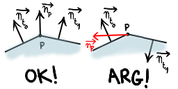
There’s a huge problem here. We are assuming that each polygon (triangle in this case) are ordered so that its normal is pointing away from the object. Unfortunately, this isn’t guaranteed by ply2 format. The following figure illustrates this.

Mesh normal problem

Imagine if t0 and t1 are coplanar. If we are in the worst case, the normals of t0 and t1 are pointing in the opposite directions. As the normal at p is the sum of those two normals, it’ll be equal to the null vector. That explains the black holes. But that’s not all… The normal at the intersection point between the ray and the triangle is interpolated from the point normals of the triangle using barycentric coordinates. One of these 3 normals may be wrong or/and, like the figure, they may be pointing in opposite directions… Arg!

There’s no exact way to determine if a polygon normal is pointing away from the surface. So, unless the file format provides polygon (or in the best case) points normals, i’ll not interpolate point normals.